[NLP] Overview of NLP

Overview of modeling Flows in NLP

In this posting, we’ll look at the overall flow of NLP. There are countless ways to perform NLP, and the flow of methodologies is changing very quickly. Therefore, it is important to understand the latest trends in NLP. Since it is difficult to handle each method in a single posting, this posting will cover only the overview of NLP, and then individual models will be covered in the subsequent postings in more detail.

• Classification by Word representation:

(** Image from: https://settlelib.tistory.com/59)

As you can see from the picture above, we can classify the methods based on word representation. Let’s take a brief look at some of the stated methods.

• One-hot Vector: So obvious. I will not explain about it. Just conduct one-hot encoding. Caution: We cannot calculate the similarities between the terms using one-hot vector.

• N-gram: An approach that considers only a few words, not all previously appeared words,. ‘N’ represents that ‘some’ word. The limitation of Statistical Language Model(SLM) is that there may not be any sentences or words in the training corpus that want to compute probabilities. N-gram was designed to alleviate this problem. N-gram means a series of N words. In the corpus you have, the model breaks it into N word bundles and considers it a token. The prediction of the next word depends only on N-1 words. The model uses conditional probabilities to decide the words that follow. The limitation of N-gram is that it sometimes can’t finish the sentence as you want since it only looks at a few words in the back.

• Bag of Words (BoW): Bag of Words is a numerical representation of text data that focuses only on the frequency of words appearing without considering the order of words at all. Let’s think of the process of making BoW as these two processes.

  (1) First, give each word a unique integer index.

  (2) Create a vector at the location of each index that records the number of appearances.

  You can use the function CountVectorizer in sklearn package to implement in python.

• TF-IDF (Term Frequency - Inverse Document Frequency): This method is not shown in the figure above, but it is one of the most popular methods in NLP. TF-IDF is a method of weighting the importance of each word within the DTM by using the frequency of the term and the inverse of frequency in documents. To use this method, we should create a DTM first, and then weights the TF-IDF. TF-IDF determines that words which appear frequently in all documents are of low importance, and words that appear frequently only in certain documents are of high importance. Measuring TF is not difficult. You can just calculate the frequency of appearance of each word in each document. The formula for calculating IDF is as follows.

  

  (** Image from: https://mungingdata.files.wordpress.com/2017/11/equation.png)

• LSA: The disadvantage of BoW-based DTM or TF-IDF was that they could not take into account the meaning of words because they were basically numerical methods using the frequency of words. As an alternative to this, a method called LSA was designed to elicit the latent meaning of DTM. The idea is that this method uses a linear algebraic method called trunked SVD for DTM or TF-IDF matrices to reduce dimensions and derive potential meanings for words. Original SVD and variations such as SVD++ will be dealt separately in separate posts later.

So far, we’ve looked at various methods used in NLP. From now on, we will review more complicated models such as GloVe, Word2Vec, BERT etc.

• Word2Vec: Since one-hot vector cannot calculate the similarity between terms, we need a way to vectorize the meaning of words to reflect the similarity between words. If we implement the method successfully, we can produce results such as Korea - Seoul + Tokyo = Japan.

  There are two methods in Word2Vec : (1) Continuous Bag of Words (CBOW) & (2) Skip-gram.

(1) CBOW: CBOW is a way of predicting the words in the middle, with the words around it. Let’s take an example.

Assume that we have a sentence “The fat cat sat on the mat” for analysis. Predicting the word “sat” from {“The”, “fat”, “cat”, “on”, “the”, “mat”} is what CBOW does. The word “sat” that should be predicted is called the center word, and the words used in the prediction are called the context word. To perform CBOW, we have to decide how many words to see in front of and behind the central word, which is called ‘window’. If the window size is 2 and the central word you want to predict is “sat”, refer to the first two words, “fat” & “cat”, and the latter two words, “on” & “the”. If you have decided the window size, you can continue to move the window to create data sets for learning by changing the surrounding and center word choices, which is called ‘sliding windows’. Be aware that all inputs should be one-hot vectors.

(2) Skip-gram: If CBOW, which was mentioned previously, predicted the central word through the peripheral word, Skip-gram predicts the peripheral word from the central word. Using the same sentence above, Skip-gram wants to predict “fat”, “cat”, “on” and “mat” through “sat”, assuming that the central word is “sat” and the window is 2. Because the logic is similar to CBOW, I guess you can easily understand it through the picture below.

(** Image from: https://wikidocs.net/22660)

• FastText: FastText is a Facebook-developed method, an extension of Word2Vec. The difference with Word2Vec is that FastText, unlike Word2Vec, it does not view words as inseparable units, but rather considers that there are multiple words in a single word. We call these words ‘subwords’. FastText treats each word as a character-wise n-gram configuration. The number of n determines how separate the words are. For example, for tri-gram with n as 3, it separates “apple” as “app”, “ppl”, and vectorize them. After learning FastText’s artificial neural network, it creates word embeddings for each n-gram of every word in the dataset. This means that if you have enough datasets, you can use the above subwords to calculate similarities with other words (Out Of Vocabulary, OOV). Also, Word2Vec had the disadvantage that embedding was not accurate for words with low frequency of appearance. However, for FastText, even if the word is a rare word, if the n-gram of the word overlaps the n-gram of the other word, it achieves a relatively high embedding vector value compared to Word2Vec. That’s why FastText has its strength in noisy corpora.

• GloVe: GloVe is a methodology that uses both count-based and predictive-based, and is a word embedding methodology developed by Stanford University in 2014. People pointed out the shortcomings of existing count-based LSA and prediction-based Word2Vec, and GloVe was devised to supplement these flaws. Actually, it turned out that GloVe’s performance is as good as Word2Vec. GloVe uses ‘window-based Co-occurrence matrix’, which is a matrix in which rows and columns are organized into words from the entire word set and the value of row i & column k is the number of times the word k appears within the given window size. ‘Co-occurrence probability’ is a conditional probability calculated by counting the total number of appearances of a particular word i from the Co-occurrence matrix and counting the number of appearances of a word k when a particular word i appears.

  To sum up GloVe’s idea in a single line, it is to make the inner product of the embedded central word and surrounding word vectors to be the probability of Co-occurence in the entire corpus. Details about GloVe like its loss function will be dealt in separate posting later.

• Seq2Seq: Seq2Seq is a model used in various fields that outputs sequences from different domains from the entered sequences. You can configure the input sequence and the output sequence as a question and answer to make it a chatbot, or you can make the input sequence and output sequence into input and translation sentences, respectively, into a translator. This is basically a model using RNN, consists of two large architectures: an ‘encoder’ and a ‘decoder’.

  The encoder receives all the words in the input sentence sequentially and then compresses all of these word information into a vector at the end, which is called the ‘context vector’. The encoder sends the context vector to the decoder when all the information in the input sentence is compressed into one context vector. The decoder receives the context vector and outputs the translated words one by one sequentially. There is not enough space to write all the relevant information, so in this posting, I will simply present a picture that shows the overall mechanism and discuss it in more detail in the next posting.

  

  (** Image from: https://wikidocs.net/images/page/24996/%EB%8B%A8%EC%96%B4%ED%86%A0%ED%81%B0%EB%93%A4%EC%9D%B4.PNG)

• ELMo (Embeddings from Language Model): It is a new word embedding methodology proposed in 2018. The biggest feature of ELMo is its use of pre-trained language models. This is why ELMo’s name contains LM. The embedding vectors expressed in Word2Vec or GloVe have the disadvantage of not properly reflecting whether the word “character” represents a text or personality. To compensate for these shortcomings, ‘Contextualized Word Embeddeding’ was created. This can be implemented through the ‘Bidirectional Language Model (biLM)’, which utilizes both language models in both directions. The biLM in ELMo basically assumes a multi-layer structure, which means that there are at least two hidden layers. The figure below shows the forward and backward language models, respectively. The interior of the encoder architecture and decoder architecture is actually two RNN architectures. RNN cells that receive input sentences are called encoders, and RNN cells that output output sentences are called decoders.

  

  (** Image from: https://wikidocs.net/images/page/33930/forwardbackwordlm2.PNG)

  Note that bi-directional RNN and biLM in ELMo are somewhat different. Unlike bi-directional RNN, where the hidden state of the forward RNN and the hidden state of the backward RNN are concatenated before sending it to the input of the next layer, biLM allows the forward and backward language models to send only the hidden state to the next layer for training.

  ELMo can be used with traditional embedding vectors. Suppose we already have an embedding vector using a method such as GloVe. Then we can concatenate ELMo representation with the GloVe embedding vector to use them as input. Then, the weights of the pre-trained language model used to create the ELMo representation are fixed. Instead, other parameters, such as the weight of each layer’s output value, are learned during the training process. The picture below explains the case precisely.

  

  (** Image from: https://wikidocs.net/images/page/33930/elmorepresentation.PNG)

• BERT (Bidirectional Encoder Representations from Transformers): As the name suggests, BERT is a model with bidirectional characteristics. Before using it, most models had a way of identifying the context by going from left to right when a sentence exists, which is naturally a limitation in grasping the entire sentence. In this respect, BERT can use bi-directionality to understand the context more naturally. Also, BERT is pre-trainable like ELMo, so you don’t need to learn from the beginning when given a specific task.

  Basically, BERT is a model that mainly uses the Transformer structure, and it uses multiple self-attention layers to extract the semantic relationships between the tokens contained in a sentence. In particular, BERT proceeds with the learning using only the encoder part. Transformer structure is a model from Google’s 2017 paper, “Attention is all you need,” which follows the encoder-decoder structure of the existing seq2seq, but is implemented only with Attention mechanism. In fact, in order to understand this structure accurately, we need to know the Attention Mechanism in detail, which we will cover in a follow-up post.

  To simply describe BERT’s algorithm, it uses Token embeddedings & Segment embeddedings & Position embeddedings to express the sentence. Token embeddedings have CLS tokens that mark the beginning of all sentences and SEP tokens that act as a separator between sentences. Segment embeddedings help make it easier to distinguish between sentences before and after, and Position embeddedings tells you where each token is located. The last embedding is the embedding used in the transformer structure, which plays an important role in enabling BERT to be bidirectional even though it is not an RNN structure. To describe it in the picture, see below.

  

  (** Image from: https://img1.daumcdn.net/thumb/R1280x0/?scode=mtistory2&fname=https%3A%2F%2Fblog.kakaocdn.net%2Fdn%2FpZneZ%2FbtqGg6mCUaU%2FEcXXk5nCUAdTRMK2vXORO0%2Fimg.png)

  BERT is a type of ‘Masked Language Model (MLM)’, which randomly masks about 15% of the input text word set. ‘Masking’ means not knowing what the original word was, and this model allows artificial neural networks to predict these masked words. BERT shows a great fit for Question & Answer / Machine Translation / Next Sentence Prediction, and has been used explosively since 2018. FYI, when fine-tuning BERT for classification problems, you can use a Dense layer with output as many as the class labels.

• XLNet: XLNet is a technology announced by the Google Research Team (Yang et al., 2019) and is an extension of the Transformer-XL (Daiet al., 2019) model that improves the Transformer Network (Vaswani et al., 2017). In Transformer-XL, ‘XL’ is ‘eXtra-Long’, which emphasizes that you can see a wider range of contexts than traditional Transformers.

  The flow of the embedding model can be divided into two main categories: AutoRegressive (AR) model and the AutoEncoding (AE) model. AR models have the limitation of not being able to see the context in both directions, and in the case of ELMo, they use both forward and reverse LSTM layers, but they are hard to see as true bidirectional models because they learn each independently. The AE model, which includes BERT, etc., is a two-way model, but there is a dependency problem between masking tokens in that the masked tokens are assumed to be independent of each other.

  Yang et al. (2019) proposed a ‘Permutation language model’ to overcome these limitations. It proceeds the model learning with randomly shuffled tokens, treating them as if they were the original order. The Permutation language model is an AR model that learns sequences sequentially, but both the two-way context of the sentence can be considered in that it is learned after performing the Permutation. Yang et al. argued that this model has bi-directionality but can overcome the disadvantages of AE model because it is AR. Also, the mismatch between pretrain-fine tuning can be solved because the masking is not done during pretraining stage. In fact, the actual implementation of the Permutation language model is realized using an attention mask, not by mixing tokens.

  Actually, XLNet has a lot of concepts that are required to understand the model from Attention mechanism to Transformer-XL and Attention mask. So if you’d like to learn more about this model, you can go to https://ratsgo.github.io/natural%20language%20processing/2019/09/11/xlnet/ and get a lot of help.

• ELECTRA: Finally, this it the last model that I want to introduce in this posting. ELECTRA is a new pre-training method that delivers the benefits of BERT, but outperforms existing technologies with the same computing budget. The model follows an efficient way of learning encoders that accurately classify token replacements, similar to the structure of GAN in the presence of generators and discriminators.

  ELECTRA trains the model using a new pre-training task called ‘Replaced Token Detection (RTD)’. As mentioned earlier, the generator and the discriminator are used to distinguish between real and fake input data, which means some input tokens are replaced with fake ones through the generator (inputs are damaged during by replacement with fake ones, unlike BERT damages them by masking) and then the discriminator part determines whether the inputs are fake or not. This structure is applied to all input tokens rather than to some mask tokens, which makes the procedure simpler and, as a result, reduces computing costs than BERT. The generator usually uses the small generator (BERT can be used), and the Discriminator part, ELECTRA, is trained to distinguish between real and fake. However, because it is difficult to apply GAN to text, it is not ‘adversarial’ in that it is trained based on maximum-likelihood. The overall structure of ELECTRA can be summarized as shown below, and other formulas or details will be discussed next time.

  

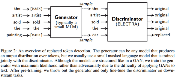
  (** Image from: https://jeonsworld.github.io/static/8a926494b114425a6772016a49a6277f/fcda8/fig2.png)

In addition to the models mentioned above, there are many other useful methods for NLP, such as ALBERT and GPT. Since we talked about the approximate flow of NLP models, I will introduce the details of each model from next time.

Upcoming…. :

Details of

• Word2Vec & FastText & GloVe
• Seq2Seq & RNN models
• ELMo & BERT & ELECTRA
• Various Distance metrics that we can use in NLP (e.g. Earth Mover Distance, Jensen-shannon Distance, Wasserstein Distance, (Soft) Cosine similarity….)

References :

• Vaswani, A., Shazeer, N., Parmar, N., Uszkoreit, J., Jones, L., Gomez, A. N., … & Polosukhin, I. (2017). Attention is all you need. arXiv preprint arXiv:1706.03762.
• Yang, Z., Dai, Z., Yang, Y., Carbonell, J., Salakhutdinov, R., & Le, Q. V. (2019). Xlnet: Generalized autoregressive pretraining for language understanding. arXiv preprint arXiv:1906.08237.

• Sutskever, I., Vinyals, O., & Le, Q. V. (2014). Sequence to sequence learning with neural networks. arXiv preprint arXiv:1409.3215.

• https://wikidocs.net/book/2155
• https://hwiyong.tistory.com/392
• https://ratsgo.github.io/natural%20language%20processing/2019/09/11/xlnet/
• https://settlelib.tistory.com/59
• https://brunch.co.kr/@synabreu/55
• https://jeonsworld.github.io/NLP/electra/