[Paper Review] Attention is all you need

Attention is all you need (2017)

In this posting, we will review a paper titled “Attention is all you need,” which introduces the attention mechanism and Transformer structure that are still widely used in NLP and other fields. BERT, which was covered in the last posting, is the typical NLP model using this attention mechanism and Transformer. Although Attention and Transformer are actively used in NLP, they are also used in many areas where recurrent methods were used. From now on, let’s take a closer look at what Attention and Transformer are.

Motivation

Until now, the recurrent models have been mainly used to analyze the sequence data. While these traditional methodologies have the advantage of maintaining the sequential nature of the data, they also have the disadvantage of long-term dependency problems. Long-term dependency problem is a problem in which two different information cannot be properly utilized since they are far from each other although those information are meaningfully close. Let’s take the sentence, “I majored in linguistics and studied deep learning in graduate school, so I became especially interested in natural language processing.”, as an example. In this case, even though the word “linguistic” plays an important role in generating the word “natural language”, the distance between the two words is not close, so the word “deep learning”(closer word) can be used to generate the word “image” instead of “natural language” when we use the recurrent models. Attention mechanism is designed to compensate for the recurrent models that have vulnerabilities in terms of long-term dependency.

In addition, the recurrent model is slow because it has to be calculated in order when learning, which implies parallelization is impossible (recently, efficiency improvement is achieved with factorization tricks and conditional computation). On the other hand, Transformer utilizing Attention mechanism has high performance since it only has to utilize attention to each word in the encoder part and masking techniques in the decoder part while training, so that the model can be parallelized.

What is attention ?

Attention is literally to pay more attention to specific information. For example, let’s say the ultimate purpose of the model is translation. Source is English(“Hi, my name is Kyoungmin”) and target is Korean(“안녕, 내 이름은 경민이야”). When the model decodes the token “이름은”, the most important thing in the source is the word “name”. So, instead of all the tokens in the source having a similar importance, “name” mush have a greater importance for better translation performance. At this point, attention is the way to make it more important.

Is it still difficult to understand the concept? That’s all right. Let’s look at the specific formula and structure of attention for detailed explanation.

• Scaled Dot-Product Attention :

  

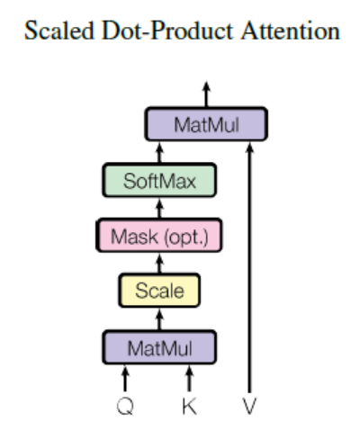
  (** Image from: https://pozalabs.github.io/assets/images/sdpa.PNG)

  The term ‘attention’ mentioned in the paper is more specifically referred to as ‘Scaled Dot-Product Attention’. The formula of Attention is as follows.

  

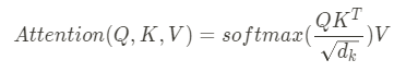
  (** Image from: https://miro.medium.com/max/372/1*1K-KmzrFUZWh5aVu61Be1g.png)

  Query(Q), Key(K), Value(V) mentioned in the above expression means:

  Query(Q) - Variables that represent the affected words / Hidden state in decoder cell at t

  Key(K) - Variables that represent words that affect / Hidden states of encoder cells at all points in time (Keys)

  Value(V) - Weight on impact / Hidden states of encoder cells at all points in time (Values)

  

  (** Image from: https://wikidocs.net/22893)

  • 1) QK^T part: The dimension of Q and K is d_k and the dimension of V is d_v. The key and value will have the same value regardless of where the attention is made. When you calculate the dot-product for the query and key, you can find the similarity between each query and key. (e.g. Cosine similarity is a similarity measure that divides the dot-product into the magnitude of the vector.)

  • 1-2) Scaling part: It is called ‘Scaled’ Dot-Product Attention because dot-product is scaled with the square root value of d_k. The reason for scaling is that the greater the value of dot-products, the less change in slope in the softmax function.

  • 2) Softmax part: After scaling, we apply softmax to get weights for values. It can be understood that this is a way to give V attention according to Q and K.

  • 3) Final multiplication part: If you multiply the result of procedure 2) to V, the final value will be higher as it is more similar to the query (which implies more important value). This fits the principle of attention - take attention to important information.

  Procedure by images (Not necessarily LSTM / Not EXACT -> Just focus on flows)

  1)

  

  2)

  

  3)

  

• Multi-Head Attention :

  

  

  

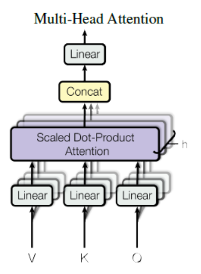
  (** Image from: https://pozalabs.github.io/transformer/ & https://i0.wp.com/rubikscode.net/wp-content/uploads/2019/08/image-7.png?resize=549%2C115&ssl=1)

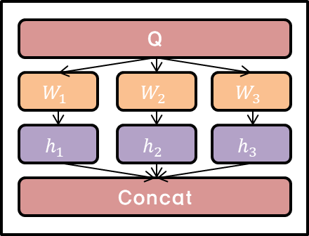
  It is better to implement different linear projections on keys, values, and queries respectively for h times than applying single attention function to d_model dimensional inputs (Reason for better performance: This procedure can reduce the size of vectors and make parallelization possible). In other words, different weight matrix W (W^Q, W^K, W^V for each i) should be multiplied to the same Q, K, and V. The projected keys, values, and queries are then passed through the attention function and then yield the value with dimension d_v.

  Then, after concatenating multiple heads, the projection is performed again, and finally a value with dimensions of d_model is derived.

  Final expression about dimensions is as follows :

  

• Self-Attention :

  

  

  I will explain the layer normalization, feed forward networks.. etc which are used after Multi-Head attention in more detail later. Since we only needs to understand the Multi-Head attention described earlier to grasp the concept of encoder part, let’s focus more on the decoder part now.

  The self-attention layer of the decoder is intended to refer only to the previous positions of the output sequence. In other words, to maintain auto-regressive properties using the i-th output as the (i+1)th input, it masks all positions after the i-th position when the attention value of i-th position is obtained. FYI, masking out means setting the input value of softmax(in attention score formula) to negative infinity.

  Masking example :

  

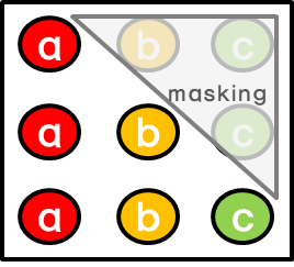
  When predicting ‘a’, attention is not given to ‘b’ and ‘c’, which are located after ‘a’. And when predicting ‘b’, attention is only given to ‘a’ (before ‘b’), and no attention is given to ‘c’ (after ‘b’).

• Encoder-Decoder Attention Layer :

  

  Queries come from the previous decoder layer and keys & values come from the output of the encoder. So in every position in the decoder, you can give attention to the input sequence, that is, to every position in the encoder output. The reason query is the output of the decoder layer is that query itself is the condition. To explain further, the question is, ‘What should be output when we have this value in decoder?’ As I explained before, the masking had already been done in decoder part, so we get attention values till i-th position through decoder.

• Position-wise Feed-Forward Networks (fully connected) :

  

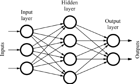
  It is ‘position-wise’ since it applies to each individual word. This network consists of two linear transformation and activation function ReLU.

  

  

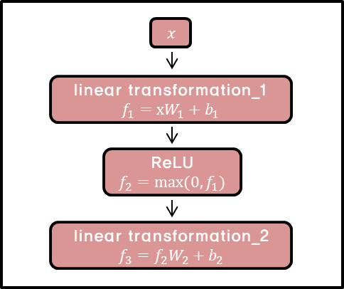
  (** Image from: https://www.programmersought.com/images/219/7c57916a929d27dd734fb3edcb367d6b.png)

  Each position uses the same parameter W,b, but if the layer changes, use a different parameter. You can also understand the above process equivalent to performing a convolution twice with kernel size 1 while treating channel as layer.

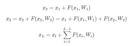
• Residual Connection :

  

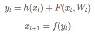
  Note that h(x_l) = x_l (-> identity mapping). You can display x_L at a particular location as the sum of x_l and the response functions as follows:

  

  After taking derivatives :

  

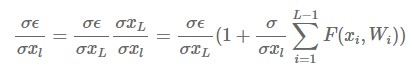
  Here we can see that the gradient value of the parent layer remains unchanged and is passed to the child layer. In other words, we can alleviate the problem of vanishing gradient - the more layers you go through, the more gradients disappear.

• Layer Normalization :

  

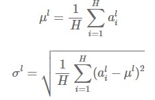
  All hidden units in the same layer share the same mu and sigma.

  

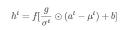
  Note that a^t = W_hh*h^(t-1) + W_xh*x^t & g,b are parameters. With this normalization, you can alleviate the problem of exploding gradient or vanishing gradient and learn faster because the gradient values become stable.

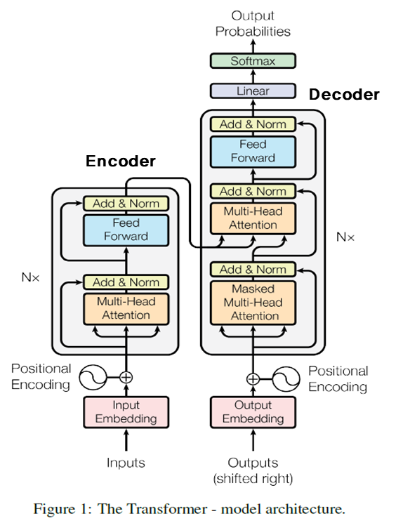
What is Transformer ?

• Model architecture :

• Positional Encoding :

  Since the transformer is neither a recurrent model nor a convolution, you need to add information about the position of the word to use the sequence of the word. So we should add positional encoding to input embedding of encoder and decoder. Note that the dimension of positional encoding is the same as that of input embedding. In the paper, the sine and cosine functions were used.

  

  

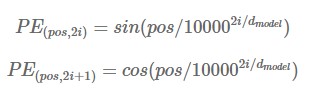
  ‘pos’ is location of the word in sequence and that certain word obtains positional encoding vector(dimension=d_model) by substituting the value from 0 to d_model/2 into i. We use cosine function when k=2i+1 and sine function when k=2i. If you get a positional encoding vector for each pos, you will have a different value if the pos is different even if it is the same column. In other words, each pos has a positional encoding value that is distinct from the other pos.

  Properties of positional encoding vector :

  

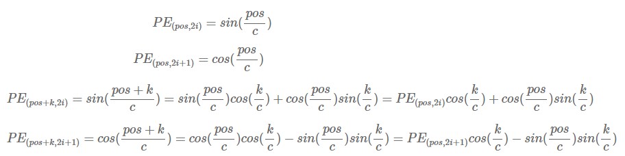
  Note that c=10000^(2i/d_model). This implies that we can express PE_(pos+k) as a linear function of PE_pos. Because of this nature, the model can learn attention more easily using relative position. The reason why we need linear transformation is that when the PE is expressed as [sin, cos, sin, cos, …] for k, PE for k+phi must be expressed as [sin, cos, sin, cos, …] too, to use the PE function at each location.

  i.e. :

  

  

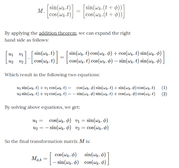
  If transformation of PE from time step k to k+phi can be obtained by linear transformation, the calculation becomes much more efficient.

• Encoder :

  Each layer has two sub-layer : multi-head self-attention mechanisms & position-wise fully connected feed-forward networks. Both 2 sub-layers use residual connection, which refers to the transmission of the input to the output. Be aware of the fact that we should align output dimension of sub-layer with embedding dimension. After that, apply layer normalization.

• Decoder :

  Decoder has a sub-layer to perform multi-head attention on the encoder’s results. It also has masked part unlike encoder, but I will skip the detailed explanation since I’ve already mentioned about it earlier. Similar to encoder part, use a residual connection for sub-layer and then implement layer normalization.

• Other details :

  Learned embedding - embedding values change during learning - was used. In addition, the learned linear transformation and softmax function were used to replace the decoder output with the probability of the next token. Using the learned linear transformation means that weight matrix W is learned, not fixed (remind that decoder output is multiplied by weight matrix W).

Conclusion

So far, we have specifically learned about Attention mechanism and Transformer through the ‘Attention is all you need’ paper review. The key point is that Attention and Transformer are presented as models that can process sequential data quickly and accurately without exploiting the recurrent. We must remember that by utilizing attention to encoders and decoders, we can emphasize the value that has the closest association with query, and parallelization has also become possible. Although a number of difficult deep learning techniques and mathematical techniques have been used, I believe that understanding these key points will make it easy for you to implement Attention mechanisms in the field.

In the next posting, we will learn more about the NLP models using attention - e.g. BERT.

Reference :

• http://www.whydsp.org/280
• http://mlexplained.com/2017/12/29/attention-is-all-you-need-explained/
• http://openresearch.ai/t/identity-mappings-in-deep-residual-networks/47
• https://m.blog.naver.com/PostView.nhn?blogId=laonple&logNo=220793640991&proxyReferer=https%3A%2F%2Fwww.google.co.kr%2F
• https://www.researchgate.net/figure/Sample-of-a-feed-forward-neural-network_fig1_234055177
• https://arxiv.org/abs/1603.05027
• https://arxiv.org/abs/1607.06450
• http://jmlr.org/papers/volume15/srivastava14a.old/srivastava14a.pdf
• https://arxiv.org/pdf/1512.00567.pdf
• https://pozalabs.github.io/transformer/
• https://hipgyung.tistory.com/12
• https://omicro03.medium.com/attention-is-all-you-need-transformer-paper-%EC%A0%95%EB%A6%AC-83066192d9ab
• https://wikidocs.net/22893