
Take baby steps towards the Computer Vision master :hammer:
Before starting, let’s define a show function. This makes your image file converted to RGB so that it appears on your jupyter notebook. (The original image is BGR)
import cv2
import matplotlib.pyplot as plt

def show(img):
    img = cv2.cvtColor(img, cv2.COLOR_BGR2RGB)
    plt.imshow(img)
    plt.axis('off')
    plt.show()
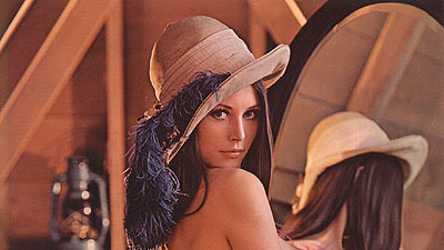
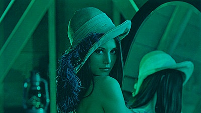
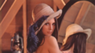
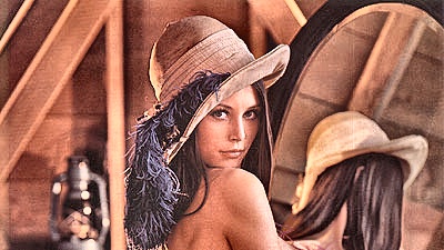
1. Load Image
fname = 'sample.jpeg'
img = cv2.imread(fname, cv2.IMREAD_COLOR) # IMREAD_COLOR: read all colors
show(img)
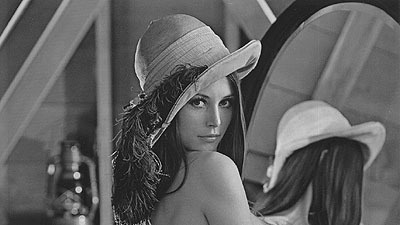
2. Gray Scaled Image
img_grey = cv2.imread(fname, cv2.IMREAD_GRAYSCALE) # read as a grey scaled pic
show(img_grey)
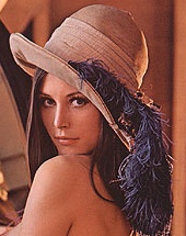
3. Resize
img_resized = cv2.resize(img, dsize=(200,100), interpolation = cv2.INTER_LINEAR)
show(img_resized)

4. Crop and Flip
img_cropped = img.copy()
img_cropped = img_cropped[10:400, 100:270]
img_cropped = cv2.flip(img_cropped, 1)
show(img_cropped)
5. Split into RGB
Well, the R, G, B channels can be divided through split function, but the splitted image looks gray since each channel is a single channel - it only looks grey but well splitted!
img_rgb = img.copy()
b, g, r = cv2.split(img_rgb)
show(b)
If you want to combine B, G only, create an empty image and merge with B and G like below.
height, width, channel = img_rgb.shape
zero = np.zeros((height, width, 1), dtype = np.uint8)
bgz = cv2.merge((b, g, zero))

show(bgz)
6. Split into HSV
HSV = Hue + Saturation + Value
img_hsv = img.copy()
img_hsv = cv2.cvtColor(img_hsv, cv2.COLOR_BGR2HSV)
h, s, v = cv2.split(img_hsv)

img1 = cv2.cvtColor(h, cv2.COLOR_BGR2RGB)
img2 = cv2.cvtColor(s, cv2.COLOR_BGR2RGB)
img3 = cv2.cvtColor(v, cv2.COLOR_BGR2RGB)

fig, ax = plt.subplots(1,3, figsize=(10,2), sharey=True)

ax[0].axis('off')
ax[1].axis('off')
ax[2].axis('off')

ax[0].imshow(img1, aspect="auto")
ax[1].imshow(img2, aspect="auto")
ax[2].imshow(img3, aspect="auto")

plt.subplots_adjust(left=0, bottom=0, right=1, top=1, wspace=0.05, hspace=0.05)

plt.show()
Basically same as #5. Convert to HSV channels and use split function.
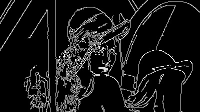
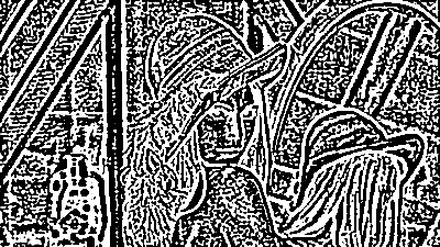
7. Laplacian filter & Canny edge detection
img_canny = img.copy()
canny = cv2.Canny(img_canny, 100, 255) # 원본 이미지 사용
laplacian = cv2.Laplacian(img_grey, cv2.CV_8U, ksize=7) # grey scaled 이미지 사용, ksize 커질 수록 더 굵어지는 느낌?
show(canny); show(laplacian)
8. Gaussian Blur
img_blur = img.copy()
img_blur = cv2.GaussianBlur(img_blur,(9,9),0)
show(img_blur)
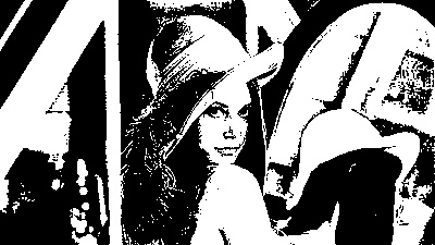
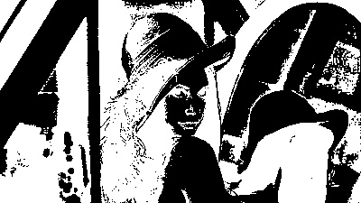
9. Threshold
img_thres = img_grey.copy()
ret, img_thres = cv2.threshold(img_thres, 100,255, cv2.THRESH_BINARY)
ret_inv, img_thres_inv = cv2.threshold(img_thres,100, 255, cv2.THRESH_BINARY_INV)
show(img_thres); show(img_thres_inv)
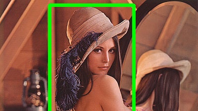
10. Boundingbox around the woman
img_box = img.copy()
img_box = cv2.rectangle(img_box, (100, 10),  (270, 250), (0, 255, 0), 5, cv2.LINE_8)
show(img_box)
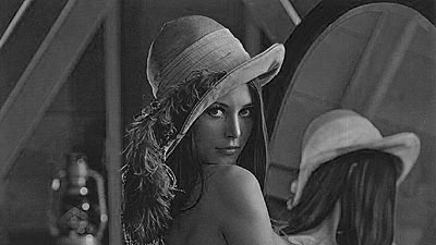
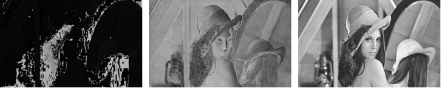
11. CLAHE (Contrast Limited Adaptive Histogram Equalization)
Image Histogram shows the distribution of pixels against its darkness. If the histogram is skewed, the image does not look good, identifiable with our naked eyes. In this case, we apply histogram equalization to equalize the distribution of darkness so that the image looks clearer. CLAHE divide the image into small titles and equialize respectively because normally an image has both bright and dark areas, so if we apply the same criteria to the whole image, the output might not be helpful for further approach.
img_clahe = img.copy()
lab = cv2.cvtColor(img_clahe, cv2.COLOR_BGR2LAB)
lab_planes = cv2.split(lab)
clahe = cv2.createCLAHE(clipLimit=2.0,tileGridSize=(8,8))
lab_planes[0] = clahe.apply(lab_planes[0])
lab = cv2.merge(lab_planes)
bgr = cv2.cvtColor(lab, cv2.COLOR_LAB2BGR)

show(bgr)
Can you tell the difference? Hopefully yes :)
12. Change the blue feather into yellow
import numpy as np

# subtract parts
img_cropped = img.copy()
img_cropped = img_cropped[50:250, 100:220]

img_feather = img.copy()
hsv = cv2.cvtColor(img_cropped, cv2.COLOR_BGR2HSV)
h, s, v = cv2.split(hsv)

# define range of blue color in HSV
lower_blue = np.array([100,50,30])
upper_blue = np.array([200,115,255])

# Threshold the HSV image to get only blue colors
mask = cv2.inRange(hsv, lower_blue, upper_blue)

# Change blue to yellow
img_cropped[mask>0]=(0, 204, 204)
img_feather[50:250, 100:220] = img_cropped
show(img_feather)
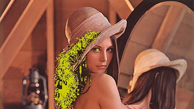
This might be tricky since you need to select the range of “blue” color to mask…
So, how to use those methods in real image data?
It might seem simple but fundamental of the computer vision. In my case, for the AI competition to detect the oral cancer, I built a function combining CLAHE and some other methods such as gamma correction. To emphasize the cancer-looking area to be more recognizable for our model, I manually tried and compared several methods. This might not seem cool but you need to know for improving your model performance :smiley:
Reference
- https://opencv-python.readthedocs.io/en/latest/doc/20.imageHistogramEqualization/imageHistogramEqualization.html